Image Processing and Computer Vision
By Golan Levin
Edited by Brannon Dorsey
This chapter introduces some basic techniques for manipulating and analyzing images in openFrameworks. As it would be impossible to treat this field comprehensively, we limit ourselves to a discussion of how images relate to computer memory, and work through an example of background subtraction, a popular operation for detecting people in video. This chapter is not a comprehensive guide to computer vision; for that, we refer you to excellent resources such as Richard Szeliski's Computer Vision: Algorithms and Applications or Gary Bradski's Learning OpenCV.
We introduce the subject "from scratch", and there's a lot to learn, so before we get started, it's worth checking to see whether there may already be a tool that happens to do exactly what you want. In the first section, we point to a few free tools that tidily encapsulate some vision workflows that are especially popular in interactive art and design.
Maybe There is a Magic Bullet
Computer vision allows you to make assertions about what's going on in images, video, and camera feeds. It's fun (and hugely educational) to create your own vision software, but it's not always necessary to implement such techniques yourself. Many of the most common computer vision workflows have been encapsulated into apps that can detect the stuff you want—and transmit the results over OSC to your openFrameworks app! Before you dig in to this chapter, consider whether you can instead sketch a prototype with one of these time-saving vision tools.
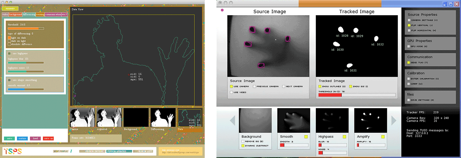
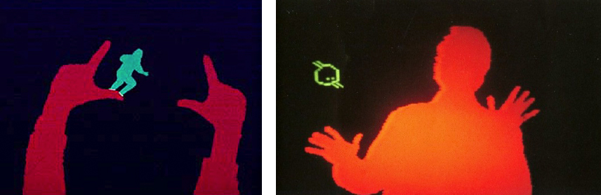
TSPS (left) and Community Core Vision (right) are richly-featured toolkits for performing computer vision tasks that are common in interactive installations. They transmit summaries of their analyses over OSC, a signalling protocol that is widely used in the media arts.
- Toolkit for Sensing People in Spaces (TSPS): A powerful toolkit for tracking bodies in video.
- Community Core Vision: Another full-featured toolkit for a wide range of tracking tasks.
- FaceOSC: An app which tracks faces (and face parts, like eyes and noses) in video, and transmits this data over OSC.
- Reactivision TUIO: A system which uses fiducial markers to track the positions and orientations of objects, and transmits this data over OSC.
- EyeOSC (.zip): An experimental, webcam-based eyetracker that transmits the viewer's fixation point over OSC.
- Synapse for Kinect: A Kinect-based skeleton tracker with OSC.
- DesignIO kinectArmTracker: A lightweight OSC app for tracking arm movements with the Kinect.
- OCR-OSC A lightweight kit for performing optical character recognition (OCR) on video streams.
This book's chapter on Game Design gives a good overview of how you can create openFrameworks apps that make use of the OSC messages generated by such tools. Of course, if these tools don't do what you need, then it's time to start reading about...
Preliminaries to Image Processing
Digital image acquisition and data structures
This chapter introduces techniques for manipulating (and extracting certain kinds of information from) raster images. Such images are sometimes also known as bitmap images or pixmap images, though we'll just use the generic term image to refer to any array (or buffer) of numbers that represent the color values of a rectangular grid of pixels ("picture elements"). In openFrameworks, such buffers come in a variety of flavors, and are used within (and managed by) a wide variety of convenient container objects, as we shall see.
Loading and Displaying an Image
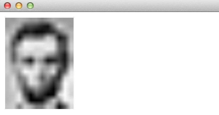
Image processing begins with, well, an image. Happily, loading and displaying an image is very straightforward in oF. Let's start with this tiny, low-resolution (12x16 pixel) grayscale portrait of Abraham Lincoln:

Below is a simple application for loading and displaying an image, very similar to the imageLoaderExample in the oF examples collection. The header file for our program, ofApp.h, declares an instance of an ofImage object, myImage:
// Example 1: Load and display an image.
// This is ofApp.h

#pragma once
#include "ofMain.h"

class ofApp : public ofBaseApp{
	public:
		void setup();
		void draw();

		// Here in the header (.h) file, we declare an ofImage:
		ofImage myImage;
};
Below is our complete ofApp.cpp file. The Lincoln image is loaded from our hard drive (once) in the setup() function; then we display it (many times per second) in our draw() function. As you can see from the filepath provided to the loadImage() function, the program assumes that the image lincoln.png can be found in a directory called "data" alongside your executable:
// Example 1: Load and display an image.
// This is ofApp.cpp

#include "ofApp.h"

void ofApp::setup(){
	// We load an image from our "data" folder into the ofImage:
	myImage.load("lincoln.png");
	myImage.setImageType(OF_IMAGE_GRAYSCALE);
}

void ofApp::draw(){
	ofBackground(255);
	ofSetColor(255);

	// We fetch the ofImage's dimensions and display it 10x larger.
	int imgWidth = myImage.getWidth();
	int imgHeight = myImage.getHeight();
	myImage.draw(10, 10, imgWidth * 10, imgHeight * 10);
}
Compiling and running the above program displays the following canvas, in which this (very tiny!) image is scaled up by a factor of 10, and rendered so that its upper left corner is positioned at pixel location (10,10). The positioning and scaling of the image are performed by the myImage.draw() command. Note that the image appears "blurry" because, by default, openFrameworks uses linear interpolation when displaying upscaled images.
If you're new to working with images in oF, it's worth pointing out that you should try to avoid loading images in the draw() or update() functions, if possible. Why? Well, reading data from disk is one of the slowest things you can ask a computer to do. In many circumstances, you can simply load all the images you'll need just once, when your program is first initialized, in setup(). By contrast, if you're repeatedly loading an image in your draw() loop — the same image, again and again, 60 times per second — you're hurting the performance of your app, and potentially even risking damage to your hard disk.
Where (Else) Images Come From
In openFrameworks, raster images can come from a wide variety of sources, including (but not limited to):
- an image file (stored in a commonly-used format like .JPEG, .PNG, .TIFF, or .GIF), loaded and decompressed from your hard drive into an
ofImage - a real-time image stream from a webcam or other video camera (using an
ofVideoGrabber) - a sequence of frames loaded from a digital video file (using an
ofVideoPlayer) - a buffer of pixels grabbed from whatever you've already displayed on your screen, captured with
ofImage::grabScreen() - a generated computer graphic rendering, perhaps obtained from an
ofFBOor stored in anofPixelsorofTextureobject - a real-time video from a more specialized variety of camera, such as a 1394b Firewire camera (via
ofxLibdc), a networked Ethernet camera (viaofxIpCamera), a Canon DSLR (usingofxCanonEOS), or with the help of a variety of other community-contributed addons likeofxQTKitVideoGrabber,ofxRPiCameraVideoGrabber, etc. - perhaps more exotically, a depth image, in which pixel values represent distances instead of colors. Depth images can be captured from real-world scenes with special cameras (such as a Microsoft Kinect via the
ofxKinectaddon), or extracted from CGI scenes using (for example)ofFBO::getDepthTexture().
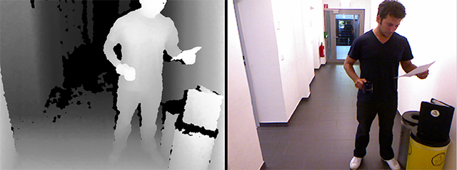
An example of a depth image (left) and a corresponding RGB color image (right), captured simultaneously with a Microsoft Kinect. In the depth image, the brightness of a pixel represents its proximity to the camera. (Note that these two images, presented in a raw state, are not yet "calibrated" to each other, meaning that there is not an exact pixel-for-pixel correspondence between a pixel's color and its corresponding depth.)
Incidentally, oF makes it easy to load images directly from the Internet, by using a URL as the filename argument, as in
myImage.load("http://en.wikipedia.org/wiki/File:Example.jpg");Keep in mind that doing this will load the remotely-stored image synchronously, meaning your program will "block" (or freeze) while it waits for all of the data to download from the web. For an improved user experience, you could instead load Internet images asynchronously (in a background thread), using the response provided by ofLoadURLAsync(); a sample implementation of this can be found in the openFrameworks imageLoaderWebExample graphics example (and check out the threadedImageLoaderExample as well). Now that you can load images stored on the Internet, you can fetch images computationally using fun APIs (like those of Temboo, Instagram or Flickr), or from dynamic online sources such as live traffic cameras.
Acquiring and Displaying a Webcam Image
The procedure for acquiring a video stream from a live webcam or digital movie file is no more difficult than loading an ofImage. The main conceptual difference is that the image data contained within an ofVideoGrabber or ofVideoPlayer object happens to be continually refreshed, usually about 30 times per second (or at the framerate of the footage). Each time you ask this object to render its data to the screen, as in myVideoGrabber.draw() below, the pixels will contain freshly updated values.
The following program (which you can find elaborated in the oF videoGrabberExample) shows the basic procedure. In this example below, for some added fun, we also retrieve the buffer of data that contains the ofVideoGrabber's pixels, then arithmetically "invert" this data (to generate a "photographic negative") and display this with an ofTexture.
The header file for our app declares an ofVideoGrabber, which we will use to acquire video data from our computer's default webcam. We also declare a buffer of unsigned chars to store the inverted video frame, and the ofTexture which we'll use to display it:
// Example 2. An application to capture, display,
// and invert live video from a webcam.
// This is ofApp.h

#pragma once
#include "ofMain.h"

class ofApp : public ofBaseApp{
	public:

		void setup();
		void update();
		void draw();

		ofVideoGrabber myVideoGrabber;
		ofTexture myTexture;

		unsigned char* invertedVideoData;
		int camWidth;
		int camHeight;
};
Does the unsigned char* declaration look unfamiliar? It's very important to recognize and understand, because this is a nearly universal way of storing and exchanging image data. The unsigned keyword means that the values which describe the colors in our image are exclusively positive numbers. The char means that each color component of each pixel is stored in a single 8-bit number—a byte, with values ranging from 0 to 255—which for many years was also the data type in which characters were stored. And the asterisk (*) means that the data named by this variable is not just a single unsigned char, but rather, an array of unsigned chars (or more accurately, a pointer to a buffer of unsigned chars). For more information about such datatypes, see the Memory in C++ chapter.
Below in Example 2 is the complete code of our webcam-grabbing .cpp file. As you might expect, the ofVideoGrabber object provides many more methods and settings, not shown here. These allow you to do things like listing and selecting available camera devices; setting your capture dimensions and framerate; and (depending on your hardware and drivers) adjusting parameters like camera exposure and contrast.
Note that the example segregates our heavy computation into the update() method, and the rendering of our graphics into draw(). This is a recommended pattern for structuring your code.
// Example 2. An application to capture, invert,
// and display live video from a webcam.
// This is ofApp.cpp

#include "ofApp.h"

void ofApp::setup(){

	// Set capture dimensions of 320x240, a common video size.
	camWidth = 320;
	camHeight = 240;

	// Open an ofVideoGrabber for the default camera
	myVideoGrabber.initGrabber (camWidth,camHeight);

	// Create resources to store and display another copy of the data
	invertedVideoData = new unsigned char [camWidth * camHeight * 3];
	myTexture.allocate (camWidth,camHeight, GL_RGB);
}

void ofApp::update(){

	// Ask the grabber to refresh its data.
	myVideoGrabber.update();

	// If the grabber indeed has fresh data,
	if(myVideoGrabber.isFrameNew()){

		// Obtain a pointer to the grabber's image data.
		unsigned char* pixelData = myVideoGrabber.getPixels().getData();

		// Reckon the total number of bytes to examine.
		// This is the image's width times its height,
		// times 3 -- because each pixel requires 3 bytes
		// to store its R, G, and B color components.
		int nTotalBytes = camWidth * camHeight * 3;

		// For every byte of the RGB image data,
		for(int i=0; i<nTotalBytes; i++){

			// pixelData[i] is the i'th byte of the image;
			// subtract it from 255, to make a "photo negative"
			invertedVideoData[i] = 255 - pixelData[i];
		}

		// Now stash the inverted data in an ofTexture
		myTexture.loadData (invertedVideoData, camWidth,camHeight, GL_RGB);
	}
}

void ofApp::draw(){
	ofBackground(100,100,100);
	ofSetColor(255,255,255);

	// Draw the grabber, and next to it, the "negative" ofTexture.
	myVideoGrabber.draw(10,10);
	myTexture.draw(340, 10);
}
This application continually displays the live camera feed, and also presents a live, "filtered" (photo negative) version. Here's the result, using my laptop's webcam:

Acquiring frames from a Quicktime movie or other digital video file stored on disk is an almost identical procedure. See the oF videoPlayerExample implementation or ofVideoGrabber documentation for details.
A common pattern among developers of interactive computer vision systems is to enable easy switching between a pre-stored "sample" video of your scene, and video from a live camera grabber. That way, you can test and refine your processing algorithms in the comfort of your hotel room, and then switch to "real" camera input when you're back at the installation site. A hacky if effective example of this pattern can be found in the openFrameworks opencvExample, in the addons example directory, where the "switch" is built using a #define preprocessor directive:
    //...
	#ifdef _USE_LIVE_VIDEO
        myVideoGrabber.initGrabber(320,240);
	#else
        myVideoPlayer.loadMovie("pedestrians.mov");
        myVideoPlayer.play();
	#endif
	//...
Uncommenting the //#define _USE_LIVE_VIDEO line in the .h file of the opencvExample forces the compiler to attempt to use a webcam instead of the pre-stored sample video.
Pixels in Memory
To begin our study of image processing and computer vision, we'll need to do more than just load and display images; we'll need to access, manipulate and analyze the numeric data represented by their pixels. It's therefore worth reviewing how pixels are stored in computer memory. Below is a simple illustration of the grayscale image buffer which stores our image of Abraham Lincoln. Each pixel's brightness is represented by a single 8-bit number, whose range is from 0 (black) to 255 (white):
In point of fact, pixel values are almost universally stored, at the hardware level, in a one-dimensional array. For example, the data from the image above is stored in a manner similar to this long list of unsigned chars:
{157, 153, 174, 168, 150, 152, 129, 151, 172, 161, 155, 156,
 155, 182, 163,  74,  75,  62,  33,  17, 110, 210, 180, 154,
 180, 180,  50,  14,  34,   6,  10,  33,  48, 106, 159, 181,
 206, 109,   5, 124, 131, 111, 120, 204, 166,  15,  56, 180,
 194,  68, 137, 251, 237, 239, 239, 228, 227,  87,  71, 201,
 172, 105, 207, 233, 233, 214, 220, 239, 228,  98,  74, 206,
 188,  88, 179, 209, 185, 215, 211, 158, 139,  75,  20, 169,
 189,  97, 165,  84,  10, 168, 134,  11,  31,  62,  22, 148,
 199, 168, 191, 193, 158, 227, 178, 143, 182, 106,  36, 190,
 205, 174, 155, 252, 236, 231, 149, 178, 228,  43,  95, 234,
 190, 216, 116, 149, 236, 187,  86, 150,  79,  38, 218, 241,
 190, 224, 147, 108, 227, 210, 127, 102,  36, 101, 255, 224,
 190, 214, 173,  66, 103, 143,  96,  50,   2, 109, 249, 215,
 187, 196, 235,  75,   1,  81,  47,   0,   6, 217, 255, 211,
 183, 202, 237, 145,   0,   0,  12, 108, 200, 138, 243, 236,
 195, 206, 123, 207, 177, 121, 123, 200, 175,  13,  96, 218};
This way of storing image data may run counter to your expectations, since the data certainly appears to be two-dimensional when it is displayed. Yet, this is the case, since computer memory consists simply of an ever-increasing linear list of address spaces.
Note how this data includes no details about the image's width and height. Should this list of values be interpreted as a grayscale image which is 12 pixels wide and 16 pixels tall, or 8x24, or 3x64? Could it be interpreted as a color image? Such 'meta-data' is specified elsewhere — generally in a container object like an ofImage.
Grayscale Pixels and Array Indices
It's important to understand how pixel data is stored in computer memory. Each pixel has an address, indicated by a number (whose counting begins with zero):
Observe how a one-dimensional list of values in memory can be arranged into successive rows of a two-dimensional grid of pixels, and vice versa.
It frequently happens that you'll need to determine the array-index of a given pixel (x,y) in an image that is stored in an unsigned char* buffer. This little task comes up often enough that it's worth committing the following pattern to memory:
// Given:
// unsigned char *buffer, an array storing a one-channel image
// int x, the horizontal coordinate (column) of your query pixel
// int y, the vertical coordinate (row) of your query pixel
// int imgWidth, the width of your image

int arrayIndex = y*imgWidth + x;

// Now you can GET values at location (x,y), e.g.:
unsigned char pixelValueAtXY = buffer[arrayIndex];

// And you can also SET values at that location, e.g.:
buffer[arrayIndex] = pixelValueAtXY;
Likewise, you can also fetch the x and y locations of a pixel corresponding to a given array index:
// Given:
// A one-channel (e.g. grayscale) image
// int arrayIndex, an index in that image's array of pixels
// int imgWidth, the width of the image

int y = arrayIndex / imgWidth; // NOTE, this is integer division!
int x = arrayIndex % imgWidth; // The friendly modulus operator.
Low-Level vs. High-Level Pixel Access Methods
Most of the time, you'll be working with image data that is stored in a higher-level container object, such as an ofImage. There are two ways to get the values of pixel data stored in such a container. In the "low-level" method, we can ask the image for a pointer to its array of raw, unsigned char pixel data, using .getPixels(), and then extract the value we want from this array. This involves some array-index calculation using the pattern described above. (And incidentally, most other openFrameworks image containers, such as ofVideoGrabber, support such a .getPixels() function.)
int arrayIndex = (y * imgWidth) + x;
unsigned char* myImagePixelBuffer = myImage.getPixels().getData();
unsigned char pixelValueAtXY = myImagePixelBuffer[arrayIndex];
The second method is a high-level function that returns the color stored at a given pixel location:
ofColor colorAtXY = myImage.getColor(x, y);
float brightnessOfColorAtXY = colorAtXY.getBrightness();
Finding the Brightest Pixel in an Image
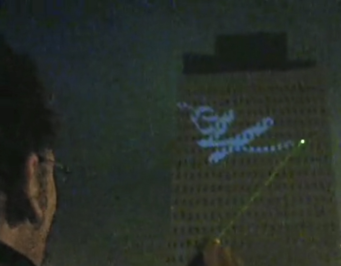
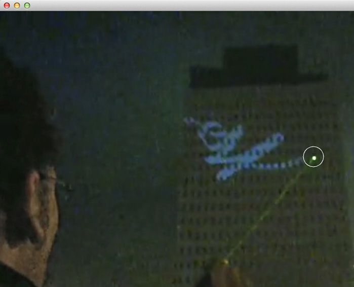
Using what we know now, we can write a simple program that locates the brightest pixel in an image. This elementary concept was used to great artistic effect by the artist collective, Graffiti Research Lab (GRL), in the openFrameworks application they built for their 2007 project L.A.S.E.R Tag. The concept of L.A.S.E.R Tag was to allow people to draw projected graffiti onto a large building facade, by means of a laser pointer. The bright spot from the laser pointer was tracked by code similar to that shown below, and used as the basis for creating interactive, projected graphics.
The .h file for our app loads an ofImage (laserTagImage) of someone pointing a laser at the building. (In the real application, a live camera was used.)
// Example 3. Finding the Brightest Pixel in an Image
// This is ofApp.h

#pragma once
#include "ofMain.h"

class ofApp : public ofBaseApp{
	public:
		void setup();
		void draw();

		// Replace this ofImage with live video, eventually
		ofImage laserTagImage;
};
Here's the .cpp file:
// Example 3. Finding the Brightest Pixel in an Image
// This is ofApp.cpp

#include "ofApp.h"

//---------------------
void ofApp::setup(){
	laserTagImage.load("images/laser_tag.jpg");
}

//---------------------
void ofApp::draw(){
	ofBackground(255);

	int w = laserTagImage.getWidth();
	int h = laserTagImage.getHeight();

	float maxBrightness = 0; // these are used in the search
	int maxBrightnessX = 0; // for the brightest location
	int maxBrightnessY = 0;

	// Search through every pixel. If it is brighter than any
	// we've seen before, store its brightness and coordinates.
	// After testing every pixel, we'll know which is brightest!
	for(int y=0; y<h; y++) {
		for(int x=0; x<w; x++) {
			ofColor colorAtXY = laserTagImage.getColor(x, y);
			float brightnessOfColorAtXY = colorAtXY.getBrightness();
			if(brightnessOfColorAtXY > maxBrightness){
				maxBrightness = brightnessOfColorAtXY;
				maxBrightnessX = x;
				maxBrightnessY = y;
			}
		}
	}

	// Draw the image.
	ofSetColor (255);
	laserTagImage.draw(0,0);

	// Draw a circle at the brightest location.
	ofNoFill();
	ofDrawEllipse (maxBrightnessX, maxBrightnessY, 40,40);
}
Our little application locates the bright spot of the laser (which, luckily for us, is the brightest part of the scene) and draws a circle around it. To reproduce L.A.S.E.R Tag, we would store the location of these points and render a light-colored trail, suitable for projection. Of course, now that we know where the brightest (or darkest) spot is, we can can develop many other interesting applications, such as sun trackers, turtle trackers...
Being able to locate the brightest pixel in an image has other uses, too. For example, in a depth image (such as produced by a Kinect sensor), the brightest pixel corresponds to the foremost point—or the nearest object to the camera. This can be extremely useful if you're making an interactive installation that tracks a user's hand.

The brightest pixel in a depth image corresponds to the nearest object to the camera. In the configuration shown here, the "nearest point" is almost certain to be the user's hand.
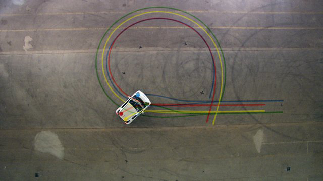
Unsurprisingly, tracking more than one bright point requires more sophisticated forms of processing. If you're able to design and control the tracking environment, one simple yet effective way to track up to three objects is to search for the reddest, greenest and bluest pixels in the scene. Zachary Lieberman used a technique similar to this in his IQ Font collaboration with typographers Pierre & Damien et al., in which letterforms were created by tracking the movements of a specially-marked sports car.
More generally, you can create a system that tracks a (single) spot with a specific color. A very simple way to achieve this is to find the pixel whose color has the shortest Euclidean distance (in "RGB space") to the target color. Here is a code fragment which shows this.
// Code fragment for tracking a spot with a certain target color.
// Our target color is CSS LightPink: #FFB6C1 or (255, 182, 193)
float rTarget = 255;
float gTarget = 182;
float bTarget = 193;

// these are used in the search for the location of the pixel
// whose color is the closest to our target color.
float leastDistanceSoFar = 255;
int xOfPixelWithClosestColor = 0;
int yOfPixelWithClosestColor = 0;

for (int y=0; y<h; y++) {
	for (int x=0; x<w; x++) {

		// Extract the color components of the pixel at (x,y)
		// from myVideoGrabber (or some other image source)
		ofColor colorAtXY = myVideoGrabber.getColor(x, y);
		float rAtXY = colorAtXY.r;
		float gAtXY = colorAtXY.g;
		float bAtXY = colorAtXY.b;

		// Compute the difference between those (r,g,b) values
		// and the (r,g,b) values of our target color
		float rDif = rAtXY - rTarget; // difference in reds
		float gDif = gAtXY - gTarget; // difference in greens
		float bDif = bAtXY - bTarget; // difference in blues

		// The Pythagorean theorem gives us the Euclidean distance.
		float colorDistance =
			sqrt (rDif*rDif + gDif*gDif + bDif*bDif);

		if(colorDistance < leastDistanceSoFar){
			leastDistanceSoFar = colorDistance;
			xOfPixelWithClosestColor = x;
			yOfPixelWithClosestColor = y;
		}
	}
}

// At this point, we now know the location of the pixel
// whose color is closest to our target color:
// (xOfPixelWithClosestColor, yOfPixelWithClosestColor)
This technique is often used with an "eyedropper-style" interaction, in which the user selects the target color interactively (by clicking). Note that there are more sophisticated ways of measuring "color distance", such as the Delta-E calculation in the CIE76 color space, that are much more robust to variations in lighting and also have a stronger basis in human color perception.
Three-Channel (RGB) Images.
Our Lincoln portrait image shows an 8-bit, 1-channel, "grayscale" image. Each pixel uses a single round number (technically, an unsigned char) to represent a single luminance value. But other data types and formats are possible.
For example, it is common for color images to be represented by 8-bit, 3-channel images. In this case, each pixel brings together 3 bytes' worth of information: one byte each for red, green and blue intensities. In computer memory, it is common for these values to be interleaved R-G-B. As you can see, RGB color images necessarily contain three times as much data.
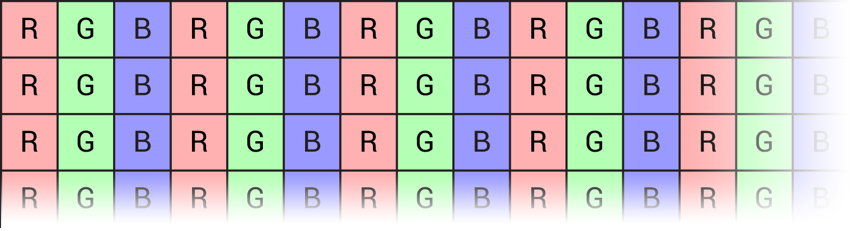
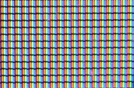
Take a very close look at your LCD screen, and you'll see how this way of storing the data is directly motivated by the layout of your display's phosphors:
Because the color data are interleaved, accessing pixel values in buffers containing RGB data is slightly more complex. Here's how you can retrieve the values representing the individual red, green and blue components of an RGB pixel at a given (x,y) location:
// Code fragment for accessing the colors located at a given (x,y)
// location in an RGB color image.

// Given:
// unsigned char *buffer, an array storing an RGB image
// (assuming interleaved data in RGB order!)
// int x, the horizontal coordinate (column) of your query pixel
// int y, the vertical coordinate (row) of your query pixel
// int imgWidth, the width of the image

int rArrayIndex = (y*imgWidth*3) + (x*3);
int gArrayIndex = (y*imgWidth*3) + (x*3) + 1;
int bArrayIndex = (y*imgWidth*3) + (x*3) + 2;

// Now you can get and set values at location (x,y), e.g.:
unsigned char redValueAtXY   = buffer[rArrayIndex];
unsigned char greenValueAtXY = buffer[gArrayIndex];
unsigned char blueValueAtXY  = buffer[bArrayIndex];
This is, then, the three-channel "RGB version" of the basic index = y*width + x pattern we employed earlier to fetch pixel values from monochrome images.
Note that you may occasionally encounter external libraries or imaging hardware which deliver RGB bytes in a different order, such as BGR.
Varieties of Image Formats
8-bit 1-channel (grayscale) and 8-bit 3-channel (RGB) images are the most common image formats you'll find. In the wide world of image processing algorithms, however, you'll eventually encounter an exotic variety of other types of images, including: - 8-bit palettized images, in which each pixel stores an index into an array of (up to) 256 possible colors; - 16-bit (unsigned short) images, in which each channel uses two bytes to store each of the color values of each pixel, with a number that ranges from 0-65535; - 32-bit (float) images, in which each color channel's data is represented by floating point numbers.
For a practical example, consider once again Microsoft's popular Kinect sensor, whose XBox 360 version produces a depth image whose values range from 0 to 1090. Clearly, that's wider than the range of 8-bit values (from 0 to 255) that one typically encounters in image data; in fact, it's approximately 11 bits of resolution. To accommodate this, the ofxKinect addon employs a 16-bit image to store this information without losing precision. Likewise, the precision of 32-bit floats is almost mandatory for computing high-quality video composites.
You'll also find:
- 2-channel images (commonly used for luminance plus transparency);
- 3-channel images (generally for RGB data, but occasionally used to store images in other color spaces, such as HSB or YUV);
- 4-channel images (commonly for RGBA images, but occasionally for CMYK);
- Bayer images, in which the RGB color channels are not interleaved R-G-B-R-G-B-R-G-B... but instead appear in a unique checkerboard pattern.
It gets even more exotic. "Hyperspectral" imagery from the Landsat 8 satellite, for example, has 11 channels, including bands for ultraviolet, near infrared, and thermal (deep) infrared!
Varieties of oF Image Containers (Data Structures)
Whereas image formats differ in the kinds of image data that they represent (e.g. 8-bit grayscale imagery vs. RGB images), image container classes are library-specific or data structures that allow their image data to be used (captured, displayed, manipulated, analyzed, and/or stored) in different ways and contexts. Some of the more common containers you may encounter in openFrameworks are:
- unsigned char* An array of unsigned chars, this is the raw, old-school, C-style format used for storing buffers of pixel data. It's not very "smart"—it has no special functionality or metadata for managing image data—but it's often useful for exchanging data between different libraries. Many image processing textbooks will assume your data is stored this way.
- ofPixels This is an openFrameworks container for pixel data which lives inside each ofImage, as well as other classes like
ofVideoGrabber. It's a wrapper around a buffer that includes additional information like width and height. - ofImage The
ofImageis the most common object for loading, saving and displaying static images in openFrameworks. Loading a file into the ofImage allocates an internalofPixelsobject to store the image data.ofImageobjects are not merely containers, but also include internal methods and objects (such as anofTexture) for displaying their pixel data to the screen. - ofxCvImage This is a container for image data used by the ofxOpenCV addon for openFrameworks, which supports a range of functionality from the popular OpenCV library for filtering, thresholding, and other image manipulations.
- ofTexture This container stores image data in the texture memory of your computer's graphics card (GPU). Many other classes, including
ofImage,ofxCvImage,ofVideoPlayer,ofVideoGrabber,ofFbo, andofKinect, maintain an internalofTextureobject to render their data to the screen. - ofFBO This is a GPU "frame buffer object", a container for textures and an optional depth buffer. It can be loosely understood as another renderer—a canvas to which you can draw 3D or 2D scenes—whose resulting pixels can themselves be treated like an image. Ultimately the
ofFBOis an object stored on the graphics card that represents a rendered drawing pass. - cv::Mat This is the data structure used by OpenCV to store image information. It's not used in openFrameworks, but if you work a lot with OpenCV, you'll often find yourself placing and extracting data from this format.
- IplImage This is an older data container (from the Intel Image Processing Library) that plays well with OpenCV. Note that you generally won't have to worry about IplImages unless (or until) you do much more sophisticated things with OpenCV; the ofxCvImage should give you everything you need to get its data in and out.
To the greatest extent possible, the designers of openFrameworks (and addons for image processing, like ofxOpenCV and Kyle McDonald's ofxCv) have provided simple operators to help make it easy to exchange data between these containers.
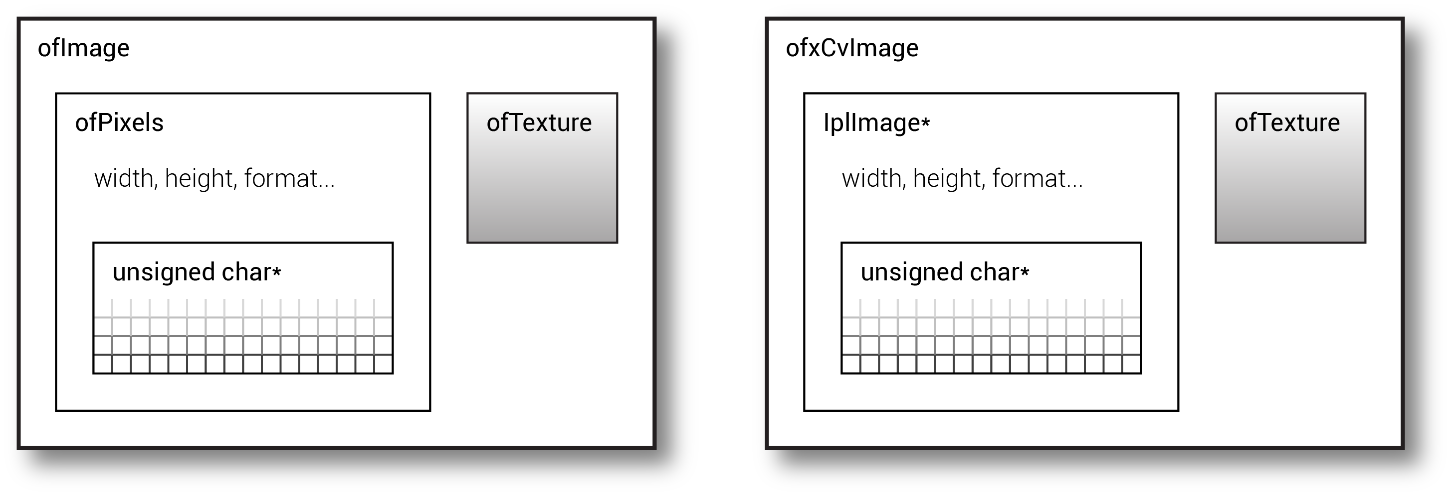
The diagram above shows a simplified representation of the two most common oF image formats you're likely to see. At left, we see an ofImage, which at its core contains an array of unsigned chars. An ofPixels object wraps up this array, along with some helpful metadata which describes it, such as its width, height, and format (RGB, RGBA, etc.). The ofImage then wraps this ofPixels object up together with an ofTexture, which provides functionality for rendering the image to the screen. The ofxCvImage at right is very similar, but stores the image data in IplImages. All of these classes provide a variety of methods for moving image data into and out of them.
It's important to point out that image data may be stored in very different parts of your computer's memory. Good old-fashioned unsigned chars, and image data in container classes like ofPixels and ofxCvImage, are maintained in your computer's main RAM; that's handy for image processing operations by the CPU. By contrast, the ofTexture class, as indicated above, stores its data in GPU memory, which is ideal for rendering it quickly to the screen. It may also be helpful to know that there's generally a performance penalty for moving image data back-and-forth between the CPU and GPU, such as the ofImage::grabScreen() method, which captures a portion of the screen from the GPU and stores it in an ofImage, or the ofTexture::readToPixels() and ofFBO::readToPixels() methods, which copy image data to an ofPixels.
RGB to Grayscale Conversion, and its Role in Computer Vision
Many computer vision algorithms (though not all) are commonly performed on one-channel (i.e. grayscale or monochrome) images. Whether or not your project uses color imagery at some point, you'll almost certainly still use grayscale pixel data to represent and store many of the intermediate results in your image processing chain. The simple fact is that working with one-channel image buffers (whenever possible) can significantly improve the speed of image processing routines, because it reduces both the number of calculations as well as the amount of memory required to process the data.
For example, if you're calculating a "blob" to represent the location of a user's body, it's common to store that blob in a one-channel image; typically, pixels containing 255 (white) designate the foreground blob, while pixels containing 0 (black) are the background. Likewise, if you're using a special image to represent the amount of motion in different parts of the video frame, it's enough to store this information in a grayscale image (where 0 represents stillness and 255 represents lots of motion). We'll discuss these operations more in later sections; for now, it's sufficient to state this rule of thumb: if you're using a buffer of pixels to store and represent a one-dimensional quantity, do so in a one-channel image buffer. Thus, except where stated otherwise, all of the examples in this chapter expect that you're working with monochrome images.
Let's suppose that your raw source data is color video (as is common with webcams). For many image processing and computer vision applications, your first step will involve converting this to monochrome. Depending on your application, you'll either clobber your color data to grayscale directly, or create a grayscale copy for subsequent processing.
The simplest method to convert a color image to grayscale is to modify its data by changing its openFrameworks image type to OF_IMAGE_GRAYSCALE. Note that this causes the image to be reallocated and any ofTextures to be updated, so it can be an expensive operation if done frequently. It's also a "destructive operation", in the sense that the image's original color information is lost in the conversion.
ofImage myImage;
myImage.load("colorful.jpg"); // Load a colorful image.
myImage.setImageType (OF_IMAGE_GRAYSCALE); // Poof! Now it's grayscale.
The ofxOpenCV addon library provides several methods for converting color imagery to grayscale. For example, the convertToGrayscalePlanarImage() and setFromColorImage() functions create or set an ofxCvGrayscaleImage from color image data stored in an ofxCvColorImage. But the easiest way is simply to assign the grayscale version from the color one; the addon takes care of the conversion for you:
// Given a color ofxOpenCv image, already filled with RGB data:
// ofxCvColorImage kittenCvImgColor;

// And given a declared ofxCvGrayscaleImage:
ofxCvGrayscaleImage kittenCvImgGray;

// The color-to-gray conversion is then performed by this assignment.
// NOTE: This uses "operator overloading" to customize the meaning of
// the '=' operator for ofxOpenCV images.
kittenCvImgGray = kittenCvImgColor;
Although oF provides the above utilities to convert color images to grayscale, it's worth taking a moment to understand the subtleties of the conversion process. There are three common techniques for performing the conversion:
- Extracting just one of the R,G, or B color channels, as a proxy for the luminance of the image. For example, one might fetch only the green values as an approximation to an image's luminance, discarding its red and blue data. For a typical color image whose bytes are interleaved R-G-B, this can be done by fetching every 3rd byte. This method is computationally fast, but it's also perceptually inaccurate, and it tends to produce noisier results for images of natural scenes.
- Taking the average of the R,G, and B color channels. A slower but more perceptually accurate method approximates luminance (often written Y) as a straight average of the red, green and blue values for every pixel:
Y = (R+G+B)/3;. This not only produces a better representation of the image's luminance across the visible color spectrum, but it also diminishes the influence of noise in any one color channel. - Computing the luminance with colorimetric coefficients. The most perceptually accurate methods for computing grayscale from color images employ a specially-weighted "colorimetric" average of the RGB color data. These methods are marginally more expensive to compute, as each color channel must be multiplied by its own perceptual weighting factor. The CCIR 601 imaging specification, which is used in the OpenCV cvtColor function, itself used in the ofxOpenCV addon, employs the formula
Y = 0.299*R + 0.587*G + 0.114*B(with the further assumption that the RGB values have been gamma-corrected). According to Wikipedia, "these coefficients represent the measured intensity perception of typical trichromat humans; in particular, human vision is most sensitive to green and least sensitive to blue."
Here's a code fragment for converting from color to grayscale, written "from scratch" in C/C++, using the averaging method described above. This code also shows, more generally, how the pixelwise computation of a 1-channel image can be based on a 3-channel image.
// Code fragment to convert color to grayscale (from "scratch")

// Load a color image, fetch its dimensions,
// and get a pointer to its pixel data.
ofImage myImage;
myImage.load ("colorful.jpg");
int imageWidth = myImage.getWidth();
int imageHeight = myImage.getHeight();
unsigned char* rgbPixelData = myImage.getPixels().getData();

// Allocate memory for storing a grayscale version.
// Since there's only 1 channel of data, it's just w*h.
int nBytesGrayscale = imageWidth * imageHeight;
unsigned char* grayPixelData = new unsigned char [nBytesGrayscale];

// For every pixel in the grayscale destination image,
for(int indexGray=0; indexGray<nBytesGrayscale; indexGray++){

	// Compute the index of the corresponding pixel in the color image,
	// remembering that it has 3 times as much data as the gray one.
	int indexColor = (indexGray * 3);

	// Fetch the red, green and blue bytes for that color pixel.
	unsigned char R = rgbPixelData[indexColor  ];
	unsigned char G = rgbPixelData[indexColor+1];
	unsigned char B = rgbPixelData[indexColor+2];

	// Compute and assign the luminance (here, as an average of R,G,B).
	// Alternatively, you could use colorimetric coefficients.
	unsigned char Y = (R+G+B)/3;
	grayPixelData[indexGray] = Y;
}
Point Processing Operations on Images
In this section, we consider image processing operations that are precursors to a wide range of further analysis and decision-making. In particular, we will look at point processing operations, namely image arithmetic and thresholding.
We begin with image arithmetic, a core part of the workflow of computer vision. These are the basic mathematical operations we all know—addition, subtraction, multiplication, and division—but as they are applied to images. Developers use such operations constantly, and for a wide range of reasons.
Image Arithmetic with Constants
Some of the simplest operations in image arithmetic transform the values in an image by a constant. In the example below, we add the constant value, 10, to an 8-bit monochrome image. Observe how the value is added pixelwise: each pixel in the resulting destination image stores a number which is 10 more (i.e. 10 gray-levels brighter) than its corresponding pixel in the source image. Because each pixel is processed in isolation, without regard to its neighbors, this kind of image math is sometimes called point processing.
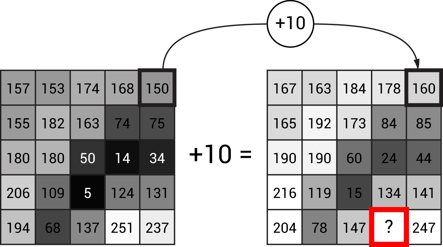
Adding a constant makes an image uniformly brighter, while subtracting a constant makes it uniformly darker.
In the code below, we implement point processing "from scratch", by directly manipulating the contents of pixel buffers. Although practical computer vision projects will often accomplish this with higher-level libraries (such as OpenCV), we do this here to show what's going on underneath.
// Example 4: Add a constant value to an image.
// This is done from "scratch", without OpenCV.
// This is ofApp.h

#pragma once
#include "ofMain.h"

class ofApp : public ofBaseApp{
	public:
	void setup();
	void draw();

	ofImage lincolnOfImageSrc; // The source image
	ofImage lincolnOfImageDst; // The destination image
};
// Example 4. Add a constant value to an image.
// This is ofApp.cpp
#include "ofApp.h"
void ofApp::setup(){
// Load the image and ensure we're working in monochrome.
// This is our source ("src") image.
lincolnOfImageSrc.load("images/lincoln_120x160.png");
lincolnOfImageSrc.setImageType(OF_IMAGE_GRAYSCALE);
// Construct and allocate a new image with the same dimensions.
// This will store our destination ("dst") image.
int imgW = lincolnOfImageSrc.getWidth();
int imgH = lincolnOfImageSrc.getHeight();
lincolnOfImageDst.allocate(imgW, imgH, OF_IMAGE_GRAYSCALE);
// Acquire pointers to the pixel buffers of both images.
// These images use 8-bit unsigned chars to store gray values.
// Note the convention 'src' and 'dst' -- this is very common.
unsigned char* srcArray = lincolnOfImageSrc.getPixels().getData();
unsigned char* dstArray = lincolnOfImageDst.getPixels().getData();
// Loop over all of the destination image's pixels.
// Each destination pixel will be 10 gray-levels brighter
// than its corresponding source pixel.
int nPixels = imgW * imgH;
for(int i=0; i<nPixels; i++) {
unsigned char srcValue = srcArray[i];
dstArray[i] = srcValue + 10;
}
// Don't forget this!
// We tell the ofImage to refresh its texture (stored on the GPU)
// from its pixel buffer (stored on the CPU), which we have modified.
lincolnOfImageDst.update();
}
//---------------------
void ofApp::draw(){
ofBackground(255);
ofSetColor(255);
lincolnOfImageSrc.draw ( 20,20, 120,160);
lincolnOfImageDst.draw (160,20, 120,160);
}A Warning about Integer Overflow
Image arithmetic is simple! But there's a lurking peril when arithmetic operations are applied to the values stored in pixels: integer overflow.
Consider what happens when we add 10 to the specially-marked pixel in the bottom row of the illustration above. Its initial value is 251—but the largest number we can store in an unsigned char is 255! What should the resulting value be? More generally, what happens if we attempt to assign a pixel value that's too large to be represented by our pixel's data type?
The answer is: it depends which libraries or programming techniques you're using, and it can have very significant consequences! Some image-processing libraries, like OpenCV, will clamp or constrain all arithmetic to the data's desired range; thus, adding 10 to 251 will result in a maxed-out value of 255 (a solution sometimes known as "saturation"). In other situations, such as with our direct editing of unsigned chars in the code above, we risk "rolling over" the data, wrapping around zero like a car's odometer. Without the ability to carry, only the least significant bits are retained. In the land of unsigned chars, adding 10 to 251 gives... 6!
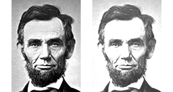
The perils of integer overflow are readily apparent in the illustration below. I have used the code above to lighten a source image of Abraham Lincoln, by adding a constant to all of its pixel values. Without any preventative measures in place, many of the light-colored pixels have "wrapped around" and become dark.

In the example above, integer overflow can be avoided by promoting the added numbers to integers, and including a saturating constraint, before assigning the new pixel value:
// The 'min' prevents values from exceeding 255, avoiding overflow.
dstArray[index] = min(255, (int)srcValue + 10);
Integer overflow can also present problems with other arithmetic operations, such as multiplication and subtraction (when values go negative).
Image Arithmetic with the ofxOpenCv Addon
The OpenCV computer vision library offers fast, easy-to-use and high-level implementations of image arithmetic. Here's the same example as above, re-written using the ofxOpenCV addon library, which comes with the openFrameworks core download. Note the following:
- ofxOpenCv provides convenient methods for copying data between images.
- ofxOpenCv provides convenient operators for performing image arithmetic.
- ofxOpenCv's arithmetic operations saturate, so integer overflow is not a concern.
- ofxOpenCv does not currently provide methods for loading images, so we employ an
ofImageas an intermediary for doing so. - As with all addons, it's important to import the ofxOpenCV addon properly into your project. (Simply adding
#include "ofxOpenCv.h"in your app's header file isn't sufficient!) The openFrameworks ProjectGenerator is designed to help you with this, and makes it easy to add an addon into a new (or pre-existing) project.
// Example 5: Add a constant value to an image, with ofxOpenCv.
// Make sure to use the ProjectGenerator to include the ofxOpenCv addon.
// This is ofApp.h
#pragma once

#include "ofMain.h"
#include "ofxOpenCv.h"

class ofApp : public ofBaseApp{
	public:
		void setup();
		void draw();
		ofxCvGrayscaleImage lincolnCvImageSrc;
		ofxCvGrayscaleImage lincolnCvImageDst;
};
// Example 5: Add a constant value to an image, with ofxOpenCv.
// This is ofApp.cpp
#include "ofApp.h"
void ofApp::setup(){
// ofxOpenCV doesn't have image loading.
// So first, load the .png file into a temporary ofImage.
ofImage lincolnOfImage;
lincolnOfImage.load("lincoln_120x160.png");
lincolnOfImage.setImageType(OF_IMAGE_GRAYSCALE);
// Set the lincolnCvImage from the pixels of this ofImage.
ofPixels & lincolnPixels = lincolnOfImage.getPixels();
lincolnCvImageSrc.setFromPixels( lincolnPixels);
// Make a copy of the source image into the destination.
lincolnCvImageDst = lincolnCvImageSrc;
// ofxOpenCV has handy operators for in-place image arithmetic.
lincolnCvImageDst += 60;
}
//---------------------
void ofApp::draw(){
ofBackground(255);
ofSetColor(255);
lincolnCvImageSrc.draw ( 20,20, 120,160);
lincolnCvImageDst.draw (160,20, 120,160);
}Here's the result. Note how the high values (light areas) have saturated instead of overflowed.
Arithmetic with Two Images: Absolute Differencing
Image arithmetic is especially useful when applied to two images. As you would expect, it is possible to add two images, multiply two images, subtract one image from another, and divide one image by another. When performing an arithmetic operation (such as addition) on two images, the operation is done "pixelwise": the first pixel of image A is added to the first pixel of image B, the second pixel of A is added to the second pixel of B, and so forth. For the purposes of this discussion, we'll assume that A and B are both monochromatic, and have the same dimensions.
Many computer vision applications depend on being able to compare two images. At the basis of doing so is the arithmetic operation of absolute differencing, illustrated below. This operation is equivalent to taking the absolute value of the results when one image is subtracted from the other: |A-B|. As we shall see, absolute differencing is a key step in common workflows like frame differencing and background subtraction.
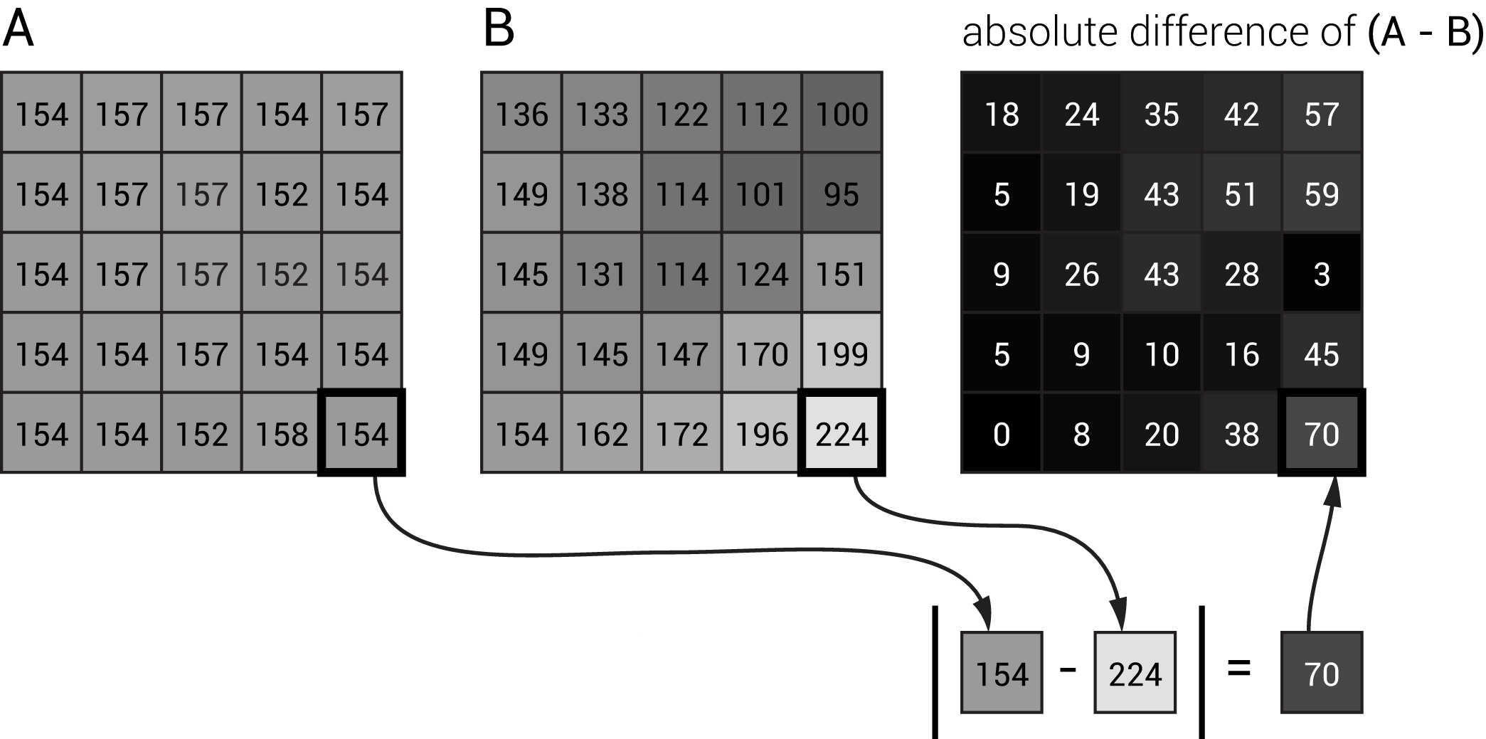
In the illustration above, we have used absolute differencing to compare two 5x5 pixel images. From this, it's clear that the greatest difference occurs in their lower-right pixels.
Absolute differencing is accomplished in just a line of code, using the ofxOpenCv addon:
// Given:
// ofxCvGrayscaleImage myCvImageA;    // the minuend image
// ofxCvGrayscaleImage myCvImageB;    // the subtrahend image
// ofxCvGrayscaleImage myCvImageDiff; // their absolute difference

// The absolute difference of A and B is placed into myCvImageDiff:
myCvImageDiff.absDiff (myCvImageA, myCvImageB);
Thresholding
In computer vision programs, we frequently have the task of determining which pixels represent something of interest, and which do not. Key to building such discriminators is the operation of thresholding.
Thresholding poses a pixelwise conditional test—that is, it asks "if" the value stored in each pixel (x,y) of a source image meets a certain criterion. In return, thresholding produces a destination image, which represents where and how the criterion is (or is not) met in the original's corresponding pixels. As we stated earlier, pixels which satisfy the criterion are conventionally assigned 255 (white), while those which don't are assigned 0 (black). And as we shall see, the white blobs which result from such thresholding are ideally suited for further analysis by contour tracers.
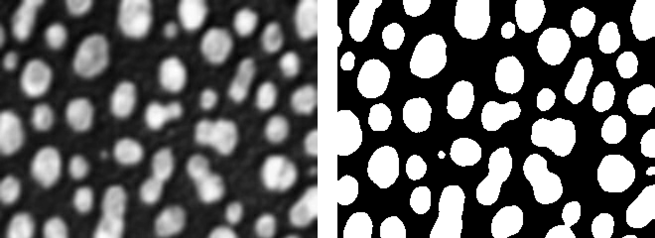
Here's an example, a photomicrograph (left) of light-colored cells. We'd like to know which pixels represent a cell, and which do not. For our criterion, we test for pixels whose grayscale brightness is greater than some constant, the threshold value. In this illustration, we test against a threshold value of 127, the middle of the 0-255 range:
And below is the complete openFrameworks program for thresholding the image—although here, instead of using a constant (127), we instead use the mouseX as the threshold value. This has the effect of placing the thresholding operation under interactive user control.
// Example 6: Thresholding
// This is ofApp.h
#pragma once

#include "ofMain.h"
#include "ofxOpenCv.h"

class ofApp : public ofBaseApp{
	public:
		void setup();
		void draw();
		ofxCvGrayscaleImage myCvImageSrc;
		ofxCvGrayscaleImage myCvImageDst;
};
// Example 6: Thresholding
// This is ofApp.cpp
#include "ofApp.h"
//---------------------
void ofApp::setup(){
// Load the cells image
ofImage cellsOfImage;
cellsOfImage.load("cells.jpg");
cellsOfImage.setImageType(OF_IMAGE_GRAYSCALE);
// Set the myCvImageSrc from the pixels of this ofImage.
ofPixels & cellsPixels = cellsOfImage.getPixels();
myCvImageSrc.setFromPixels (cellsPixels);
}
//---------------------
void ofApp::draw(){
ofBackground(255);
ofSetColor(255);
// Copy the source image into the destination:
myCvImageDst = myCvImageSrc;
// Threshold the destination image.
// Our threshold value is the mouseX,
// but it could be a constant, like 127.
myCvImageDst.threshold (mouseX);
myCvImageSrc.draw ( 20,20, 320,240);
myCvImageDst.draw (360,20, 320,240);
}A Complete Workflow: Background Subtraction
We now have all the pieces we need to understand and implement a popular and widely-used workflow in computer vision: contour extraction and blob tracking from background subtraction. This workflow produces a set of (x,y) points that represent the boundary of (for example) a person's body that has entered the camera's view.
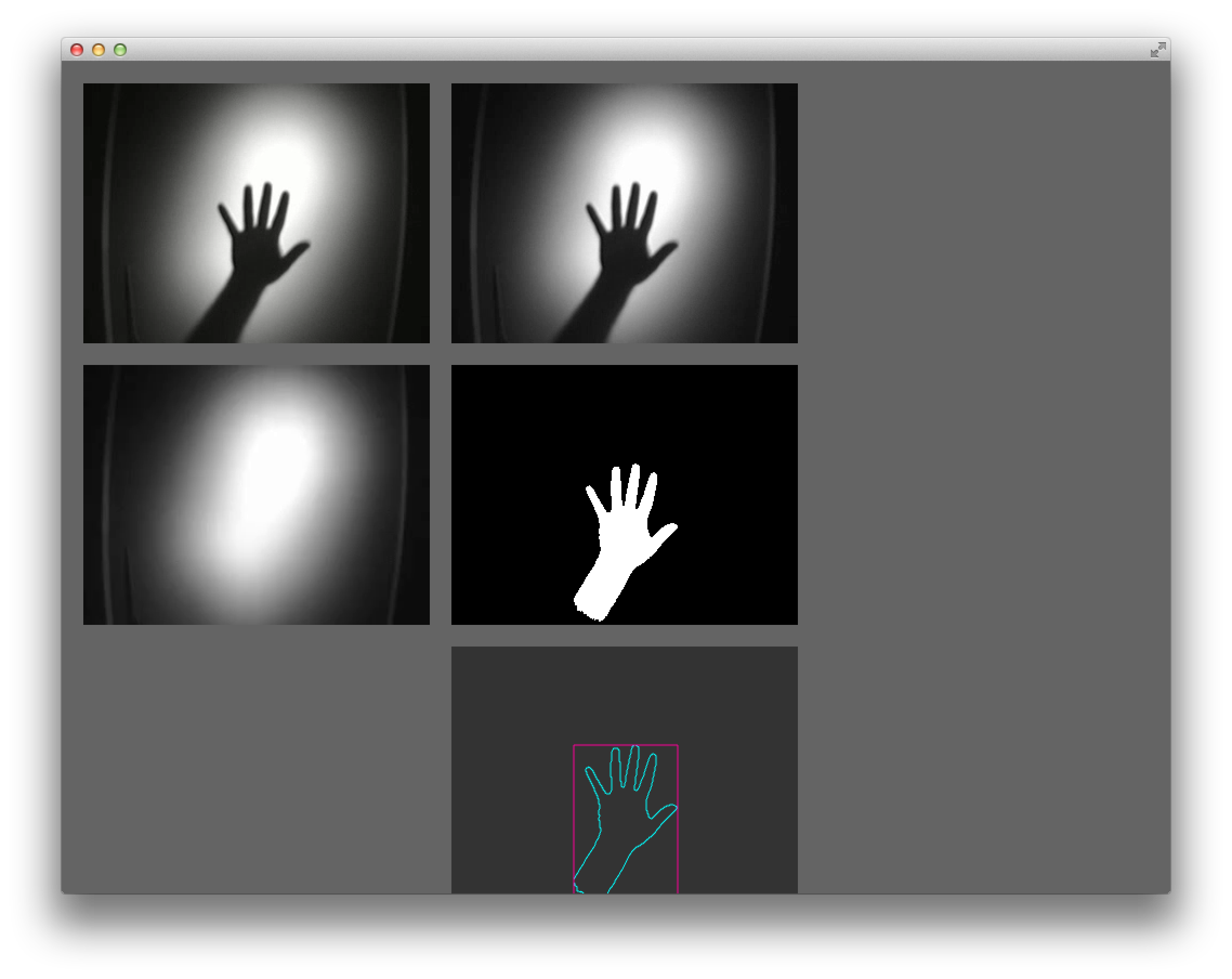
In this section, we'll base our discussion around the standard openFrameworks opencvExample, which can be found in the examples/addons/opencvExample directory of your openFrameworks installation. When you compile and run this example, you'll see a video of a hand casting a shadow—and, at the bottom right of our window, the contour of this hand, rendered as a cyan polyline. This polyline is our prize: using it, we can obtain all sorts of information about our visitor. So how did we get here?
The code below is a slightly simplified version of the standard opencvExample; for example, we have here omitted some UI features, and we have omitted the #define _USE_LIVE_VIDEO (mentioned earlier) which allows for switching between a live video source and a stored video file.
In the discussion that follows, we separate the inner mechanics into five steps, and discuss how they are performed and displayed:
- Video Acquisition
- Color to Grayscale Conversion
- Storing a "Background Image"
- Thresholded Absolute Differencing
- Contour Tracing
// Example 7: Background Subtraction
// This is ofApp.h

#pragma once
#include "ofMain.h"
#include "ofxOpenCv.h"

class ofApp : public ofBaseApp{
	public:
		void setup();
		void update();
		void draw();
		void keyPressed(int key);

		ofVideoPlayer			vidPlayer;

		ofxCvColorImage			colorImg;
		ofxCvGrayscaleImage 	grayImage;
		ofxCvGrayscaleImage 	grayBg;
		ofxCvGrayscaleImage 	grayDiff;
		ofxCvContourFinder		contourFinder;

		int						thresholdValue;
		bool					bLearnBackground;
};
// Example 7: Background Subtraction
// This is ofApp.cpp
#include "ofApp.h"
//---------------------
void ofApp::setup(){
vidPlayer.load("fingers.mov");
vidPlayer.play();
colorImg.allocate(320,240);
grayImage.allocate(320,240);
grayBg.allocate(320,240);
grayDiff.allocate(320,240);
bLearnBackground = true;
thresholdValue = 80;
}
//---------------------
void ofApp::update(){
// Ask the video player to update itself.
vidPlayer.update();
if (vidPlayer.isFrameNew()){ // If there is fresh data...
// Copy the data from the video player into an ofxCvColorImage
colorImg.setFromPixels(vidPlayer.getPixels());
// Make a grayscale version of colorImg in grayImage
grayImage = colorImg;
// If it's time to learn the background;
// copy the data from grayImage into grayBg
if (bLearnBackground == true){
grayBg = grayImage; // Note: this is 'operator overloading'
bLearnBackground = false; // Latch: only learn it once.
}
// Take the absolute value of the difference
// between the background and incoming images.
grayDiff.absDiff(grayBg, grayImage);

// Perform an in-place thresholding of the difference image.
grayDiff.threshold(thresholdValue);
// Find contours whose areas are betweeen 20 and 25000 pixels.
// "Find holes" is true, so we'll also get interior contours.
contourFinder.findContours(grayDiff, 20, 25000, 10, true);
}
}
//---------------------
void ofApp::draw(){
ofBackground(100,100,100);
ofSetHexColor(0xffffff);
colorImg.draw(20,20); // The incoming color image
grayImage.draw(360,20); // A gray version of the incoming video
grayBg.draw(20,280); // The stored background image
grayDiff.draw(360,280); // The thresholded difference image
ofNoFill();
ofDrawRectangle(360,540,320,240);
// Draw each blob individually from the blobs vector
int numBlobs = contourFinder.nBlobs;
for (int i=0; i<numBlobs; i++){
contourFinder.blobs[i].draw(360,540);
}
}
//---------------------
void ofApp::keyPressed(int key){
bLearnBackground = true;
}Step 1. Video Acquisition.
In the upper-left of our screen display is the raw, unmodified video of a hand creating a shadow. Although it's not very obvious, this is actually a color video; it just happens to be showing a mostly black-and-white scene.
In setup(), we initialize some global-scoped variables (declared in ofApp.h), and allocate the memory we'll need for a variety of globally-scoped ofxCvImage image buffers. We also load the hand video from from its source file into vidPlayer, a globally-scoped instance of an ofVideoPlayer.
It's quite common in computer vision workflows to maintain a large number of image buffers, each of which stores an intermediate state in the image-processing chain. For optimal performance, it's best to allocate() these only once, in setup(); otherwise, the operation of reserving memory for these images can hurt your frame rate.
Here, the colorImg buffer (an ofxCvColorImage) stores the unmodified color data from vidPlayer; whenever there is a fresh frame of data from the player, in update(), colorImg receives a copy. Note the commands by which the data is extracted from vidPlayer and then assigned to colorImg:
colorImg.setFromPixels(vidPlayer.getPixels());In the full code of opencvExample (not shown here) a #define near the top of ofApp.h allows you to swap out the ofVideoPlayer for an ofVideoGrabber—a live webcam.
Step 2. Color to Grayscale Conversion.
In the upper-right of the window is the same video, converted to grayscale. Here it is stored in the grayImage object, which is an instance of an ofxCvGrayscaleImage.
It's easy to miss the grayscale conversion; it's done implicitly in the assignment grayImage = colorImg; using operator overloading of the = sign. All of the subsequent image processing in opencvExample is done with grayscale (rather than color) images.
Step 3. Storing a "Background Image".
In the middle-left of the screen is a view of the background image. This is a grayscale image of the scene that was captured, once, when the video first started playing—before the hand entered the frame.
The background image, grayBg, stores the first valid frame of video; this is performed in the line grayBg = grayImage;. A boolean latch (bLearnBackground) prevents this from happening repeatedly on subsequent frames. However, this latch is reset if the user presses a key.
It is absolutely essential that your system "learn the background" when your subject (such as the hand) is out of the frame. Otherwise, your subject will be impossible to detect properly!
Step 4. Thresholded Absolute Differencing.
4. In the middle-right of the screen is an image that shows the thresholded absolute difference between the current frame and the background frame. The white pixels represent regions that are significantly different from the background: the hand!
The absolute differencing and thresholding take place in two separate operations, whose code is shown below. The absDiff() operation computes the absolute difference between grayBg and grayImage (which holds the current frame), and places the result into grayDiff.
The subsequent thresholding operation ensures that this image is binarized, meaning that its pixel values are either black (0) or white (255). The thresholding is done as an in-place operation on grayDiff, meaning that the grayDiff image is clobbered with a thresholded version of itself.
The variable thresholdValue is set to 80, meaning that a pixel must be at least 80 gray-levels different than the background in order to be considered foreground. In the official example, a keypress permits the user to adjust this number.
// Take the absolute value of the difference
// between the background and incoming images.
grayDiff.absDiff(grayBg, grayImage);
// Perform an in-place thresholding of the difference image.
grayDiff.threshold(thresholdValue);This example uses thresholding to distinguish dark objects from a light background. But it's worth pointing out that thresholding can be applied to any image whose brightness quantifies a variable of interest.
If you're using a webcam instead of the provided "fingers.mov" demo video, note that automatic gain control can sometimes interfere with background subtraction. You may need to increase the value of your threshold, or use a more sophisticated background subtraction technique.
Step 5. Contour Tracing.
5. The final steps are displayed in the bottom right of the screen. Here, an ofxCvContourFinder has been tasked to findContours() in the binarized image. It does this by identifying contiguous blobs of white pixels, and then tracing the contours of those blobs into an ofxCvBlob outline comprised of (x,y) points.
Internally, the ofxCvContourFinder first performs a pixel-based operation called connected component labeling, in which contiguous areas are identified as uniquely-labeled blobs. It then extracts the boundary of each blob, which it stores in an ofPolyline, using a process known as a chain code algorithm.
Some of the parameters to the findContours() method allow you to select only those blobs which meet certain minimum and maximum area requirements. This is useful if you wish to discard very tiny blobs (which can result from noise in the video) or extremely large blobs (which can result from sudden changes in lighting).
// Find contours whose areas are betweeen 20 and 25000 pixels.
// "Find holes" is set to true, so we'll also get interior contours.
contourFinder.findContours(grayDiff, 20, 25000, 10, true);
In draw(), the app then displays the contour of each blob in cyan, and also shows the bounding rectangle of those points in magenta.
// Draw each blob individually from the blobs vector
int numBlobs = contourFinder.nBlobs;
for (int i=0; i<numBlobs; i++){
   contourFinder.blobs[i].draw(360,540);
}
Frame Differencing
Closely related to background subtraction is frame differencing. If background subtraction is useful for detecting presence (by comparing a scene before and after someone entered it), frame differencing is useful for detecting motion.
The difference between background subtraction and frame differencing can be described as follows:
- Background subtraction compares the current frame with a previously-stored background image
- Frame differencing compares the current frame with the immediately previous frame of video.
As with background subtraction, it's customary to threshold the difference image, in order to discriminate signals from noise. Using frame differencing, it's possible to quantify how much motion is happening in a scene. This can be done by counting up the white pixels in the thresholded difference image.
In practice, background subtraction and frame differencing are often used together. For example, background subtraction can tell us that someone is in the room, while frame differencing can tell us how much they are moving around. In a common solution that combines the best of both approaches, motion detection (from frame differencing) and presence detection (from background subtraction) can be combined to create a generalized detector. A simple trick for doing so is to take a weighted average of their results, and use that as the basis for further thresholding.
Contour Games
Blob contours are a vector-based representation, comprised of a series of (x,y) points. Once obtained, a contour can be used for all sorts of exciting geometric play.
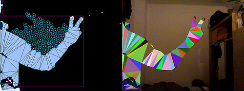
A good illustration of this is the following project by Cyril Diagne, in which the body's contour is triangulated by ofxTriangle, and then used as the basis for simulated physics interactions using ofxBox2D. The user of Diagne's project can "catch" the bouncy circular "balls" with their silhouette.
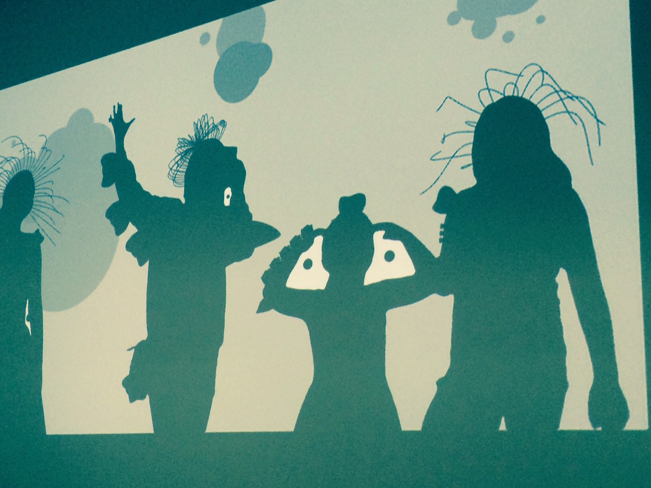
One of the flags to the ofxCvContourFinder::findContours() function allows you to search specifically for interior contours, also known as negative space. An interactive artwork which uses this to good effect is Shadow Monsters by Philip Worthington, which interprets interior contours as the boundaries of lively, animated eyeballs.
The original masterwork of contour play was Myron Krueger’s landmark interactive artwork, Videoplace, which was developed continuously between 1970 and 1989, and which premiered publicly in 1974. The Videoplace project comprised at least two dozen profoundly inventive scenes which comprehensively explored the design space of full-body camera-based interactions with virtual graphics — including telepresence applications and (as pictured here, in the “Critter” scene) interactions with animated artificial creatures.
Here's a quick list of some fun and powerful things you can do with contours extracted from blobs:
- A blob's contour is represented as a
ofPolyline, and can be smoothed and simplified withofPolyline::getSmoothed(). Try experimenting with extreme smoothing, to create ultra-filtered versions of captured geometry. - If you have too many (or too few) points in your contour, consider using
ofPolyline::getResampledBySpacing()orgetResampledByCount()to reduce (or increase) its number of points. ofPolylineprovides methods for computing the area, perimeter, centroid, and bounding box of a contour; consider mapping these to audiovisual or other interactive properties. For example, you could map the area of a shape to its mass (in a physics simulation), or to its color.- You can identify "special" points on a shape (such as the corners of a square, or an extended fingertip on a hand) by searching through a contour for points with high local curvature. The function
ofPolyline::getAngleAtIndex()can be helpful for this. - The mathematics of shape metrics can provide powerful tools for contour analysis and even recognition. One simple shape metric is aspect ratio, which is the ratio of a shape's width to its height. Another elegant shape metric is compactness (also called the isoperimetric ratio), which the ratio of a shape's perimeter-squared to its area. You can use these metrics to distinguish between (for example) cardboard cutouts of animals or numbers.
- The ID numbers (array indices) assigned to blobs by the
ofxCvContourFinderare based on the blobs' sizes and locations. If you need to track multiple blobs whose positions and areas change over time, see the example-contours-tracking example in Kyle McDonald's addon, ofxCv.
Refinements
In this section we briefly discuss several important refinements that can be made to improve the quality and performance of computer vision programs.
- Cleaning Up Thresholded Images: Erosion and Dilation
- Automatic Thresholding and Dynamic Thresholding
- Adaptive Background Subtraction
- ROI Processing
Cleaning Up Thresholded Images: Erosion and Dilation
Sometimes thresholding leaves noise, which can manifest as fragmented blobs or unwanted speckles. If altering your threshold value doesn't solve this problem, you'll definitely want to know about erosion and dilation, which are types of morphological operators for binarized images. Simply put,
- Erosion removes a layer of pixels from every blob in the scene.
- Dilation adds a layer of pixels to every blob in the scene.
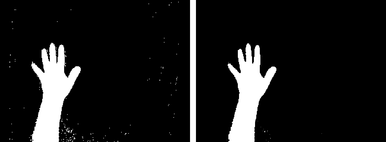
In the example below, one pass of erosion is applied to the image at left. This eliminates all of the isolated specks of noise:
By contrast, observe how dilation is used in the person-detecting pipeline below:
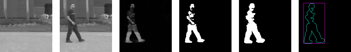
- Live video is captured and converted to grayscale. A background image is acquired at a time when nobody is in the scene. (Sometimes, a running average of the camera feed is used as the background, especially for outdoor scenes subject to changing lighting conditions.)
- A person walks into the frame.
- The live video image is compared with the background image. The absolute difference of Images (1) and (2) is computed.
- Image (3), the absolute difference, is thresholded. Unfortunately, the person's body is fragmented into pieces, because some pixels were insufficiently different from the background.
- Two passes of dilation are applied to Image (4) the thresholded image. This fills in the cracks between the pieces, creating a single, contiguous blob.
- The contour tracer identifies just one blob instead of several.
OpenCV makes erosion and dilation easy. See ofxCvImage::erode() and ofxCvImage::dilate() for methods that provide access to this functionality.
Other operations which may be helpful in removing noise is ofxCvImage::blur() and ofxCvImage:: blurGaussian(). These should be applied before the thresholding operation, rather than after.
Adaptive Background Subtraction
In situations with fluctuating lighting conditions, such as outdoor scenes, it can be difficult to perform background subtraction. One common solution is to slowly adapt the background image over the course of the day, accumulating a running average of the background.
The overloaded operators for ofxCvImage make such running averages straightforward. In the code fragment below, the background image is continually but slowly reassigned to be a combination of 99% of what it was a moment ago, with 1% of new information. This is also known as an adaptive background.
grayBg = 0.99*grayBg + 0.01*grayImage;Automatic Thresholding and Dynamic Thresholding
Sometimes it's difficult to know in advance exactly what the threshold value should be. Camera conditions change, lighting conditions change, scene conditions change; all affect the value which we hope to use to distinguish light from dark.
To resolve this, you could make this a manually adjusted setting, as we did in Example 6 (above) when we used the mouseX as the threshold value. But there are also automatic thresholding techniques that can compute an "ideal" threshold based on an image's luminance histogram. There are dozens of great techniques for this, including Otsu's Method, Gaussian Mixture Modeling, IsoData Thresholding, and Maximum Entropy thresholding. For an amazing overview of such techniques, check out ImageJ, an open-source (Java) computer vision toolkit produced by the US National Institute of Health.
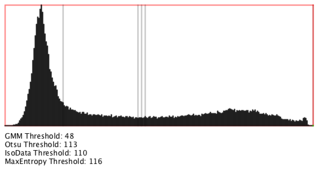
Below is code for the Isodata method, one of the simpler (and shorter) methods for automatically computing an ideal threshold. Note that the function takes as input the image's histogram: an array of 256 integers that contain the count, for each gray-level, of how many pixels are colored with that gray-level.
/*
From: http://www.ph.tn.tudelft.nl/Courses/FIP/frames/fip-Segmenta.html
This iterative technique for choosing a threshold was developed by
Ridler and Calvard. The histogram is initially segmented into two parts
using a starting threshold value such as th0 = 127, half the maximum
dynamic range for an 8-bit image. The sample mean (mf,0) of the gray
values associated with the foreground pixels and the sample mean (mb,0)
of the gray values associated with the background pixels are computed.
A new threshold value th1 is now computed as the average of these two
sample means. The process is repeated, based upon the new threshold,
until the threshold value does not change any more.

Input: imageHistogram, an array of 256 integers, each of which represents
the count of pixels that have that particular gray-level. For example,
imageHistogram[56] contains the number of pixels whose gray-level is 56.
Output: an integer (between 0-255) indicating an ideal threshold.
*/

int ofApp::getThresholdIsodata (int *imageHistogram){
	int theThreshold = 127; // our output

	if (input != NULL){ // sanity check
		int thresh = theThreshold;
		int tnew = thresh;
		int thr  = 0;
		int sum  = 0;
		int mean1, mean2;
		int ntries = 0;

		do {
			thr = tnew;
			sum = mean1 = mean2 = 0;

			for (int i=0; i<thr; i++){
				mean1 += (imageHistogram[i] * i);
				sum   += (imageHistogram[i]);
			}
			if (sum != 0){ mean1 = mean1 / sum;}

			sum = 0;
			for (int i=thr; i<255; i++){
				mean2 += (imageHistogram[i] * i);
				sum   += (imageHistogram[i]);
			}

			if (sum != 0){ mean2 = mean2 / sum;}
			tnew = (mean1 + mean2) / 2;
			ntries++;

		} while ((tnew != thr) && (ntries < 64));
		theThreshold = tnew;
	}
	return theThreshold;
}
In some situations, such as images with strong gradients, a single threshold may be unsuitable for the entire image field. Instead, it may be preferable to implement some form of per-pixel thresholding, in which a different threshold is computed for every pixel (i.e. a "threshold image").
As you can see below, a single threshold fails for this particular source image, a page of text. Instead of using a single number, the threshold is established for each pixel by taking an average of the brightness values in its neighborhood (minus a constant!).
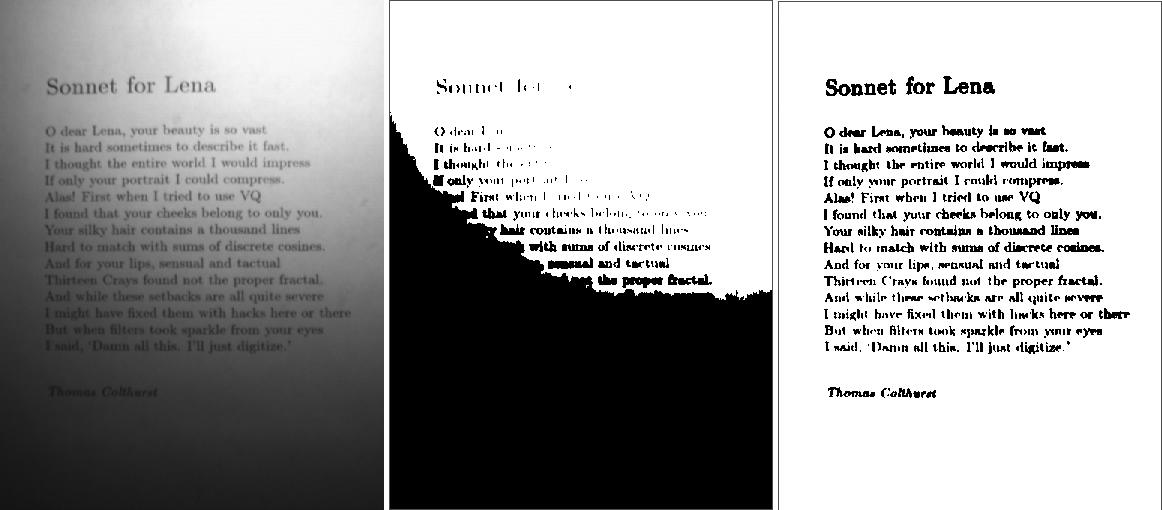
The name for this technique is adaptive thresholding, and an excellent discussion can be found in the online Hypertext Image Processing Reference.
ROI Processing
Many image processing and computer vision operations can be sped up by performing calculations only within a sub-region of the main image, known as a region of interest or ROI.
The relevant function is ofxCvImage::setROI(), which sets the ROI in the image. Region of Interest is a rectangular area in an image, to segment object for further processing. Once the ROI is defined, OpenCV functions will operate on the ROI, reducing the number of pixels that the operation will examine and modify.
Suggestions for Further Experimentation
There's tons more to explore! We strongly recommend you try out all of the openCV examples that come with openFrameworks. (An audience favorite is the opencvHaarFinderExample, which implements the classic Viola-Jones face detector!) When you're done with those, check out the examples that come with Kyle McDonald's ofxCv addon.
I sometimes assign my students the project of copying a well-known work of interactive new-media art. Reimplementing projects such as the ones below can be highly instructive, and test the limits of your attention to detail. Such copying provides insights which cannot be learned from any other source. I recommend you build...
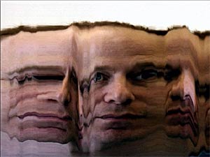
A Slit-Scanner.
Slit-scanning — a type of spatiotemporal or "time-space imaging" — has been a common trope in interactive video art for more than twenty years. Interactive slit-scanners have been developed by some of the most revered pioneers of new media art (Toshio Iwai, Paul de Marinis, Steina Vasulka) as well as by literally dozens of other highly regarded practitioners. The premise remains an open-ended format for seemingly limitless experimentation, whose possibilities have yet to be exhausted. It is also a good exercise in managing image data, particularly in extracting and copying image subregions.
In digital slit-scanning, thin slices are extracted from a sequence of video frames, and concatenated into a new image. The result is an image which succinctly reveals the history of movements in a video or camera stream. In Time Scan Mirror (2004) by Danny Rozin, for example, a image is composed from thin vertical slices of pixels that have been extracted from the center of each frame of incoming video, and placed side-by-side. Such a slit-scanner can be built in fewer than 20 lines of code—try it!
A cover of Text Rain by Utterback & Achituv (1999).
Text Rain by Camille Utterback and Romy Achituv is a now-classic work of interactive art in which virtual letters appear to "fall" on the visitor's "silhouette". Utterback writes: "In the Text Rain installation, participants stand or move in front of a large projection screen. On the screen they see a mirrored video projection of themselves in black and white, combined with a color animation of falling letters. Like rain or snow, the letters appears to land on participants’ heads and arms. The letters respond to the participants’ motions and can be caught, lifted, and then let fall again. The falling text will 'land' on anything darker than a certain threshold, and 'fall' whenever that obstacle is removed."

Text Rain can be implemented in about 30 lines of code, and involves many of the topics we've discussed in this chapter, such as fetching the brightness of a pixel at a given location. It can also be an ideal project for ensuring that you understand how to make objects (to store the positions and letters of the falling particles) and arrays of objects.
========================================================
## Bibliography
This chapter has introduced a few introductory image processing and computer vision techniques. But computer vision is a huge and constantly evolving field. For more information, we highly recommend the following books and online resources.
- Bradski, Gary. Learning OpenCV (PDF)
- Cardoso, Jorge. Computer vision techniques for interactive art
- Fisher, Robert, et. al. HIPR2, The Hypertext Image Processing Reference
- Introduction to Video and Image Processing
- Levin, Golan. Computer Vision for Artists and Designers
- Szeliski & Zisserman. 20 techniques that every computer vision researcher should know (PDF)
- Szeliski, Richard. Computer Vision: Algorithms and Applications
- The OpenCV Reference Manual (PDF)